SimulateMixin

class cait.mixins.SimulateMixin

Bases: object

A Mixin Class for the DataHandler class with methods to simulate data sets.

efficiency_sim_trigger_of(sim_ts: ndarray, sim_phs: ndarray, stream: StreamBaseClass, trigger_channels: str | List[str], of: ndarray, thresholds: float | List[float], sev: ndarray = None, sev_fitpars: List[List[float]] = None, shift_samples: List[List[int]] = None, shift_subsamples: List[List[float]] = None, passive_channels: str | List[str] = None, testpulse_channels: str | List[str] = None, tolerance_samples: int = 10, n_record_lens: int = 8, record_placement: int = 4, tag: str = '', preview: bool = False)

Perform a trigger efficiency simulation by superimposing a SEV onto random parts of a stream and running an optimum filter trigger to check whether they survive or not. See below for a description of the algorithm.

The trigger-specific arguments to this function correspond to the ones of cait.mixins.TriggerCollectionMixin.trigger_of(), and the two are meant to be used in combination (i.e. the trigger efficiency function mimics the behavior of the trigger function). The arguments that the trigger function has but which are not featured here are irrelevant for the efficiency. Also refer to cait.mixins.TriggerCollectionMixin.trigger_of() for more information.

Parameters:

• sim_ts (np.ndarray) – The timestamps at which you want to simulate events. These cannot be within the first nor the last two record windows of the stream (because there, the filtering is unreliable). This is a 1d-array, i.e. even if you simulate pulses on multiple channels, they are simulated at identical timestamps. Events are simulated such that the SEV of the first trigger channel has its maximum at the given timestamp.

• sim_phs (np.ndarray) – The pulse heights of the pulses that you want to simulate. This has to have as many rows as there are trigger and passive channels (i.e. we simulate pulses on all channels which are of interest).

• stream (StreamBaseClass) – The stream object including the channels that you want to trigger.

• trigger_channels (List[Union[Tuple[str], str]]) – The list of channel names to be triggered. Have to be present in stream.keys. If you pass a tuple of channel names, the 2D optimum filter is applied to this combination.

• of (np.ndarray) – The optimum filter to use for triggering (Has to have one for each channel in trigger_channels. If either of the trigger channels is a tuple, i.e. treated using the 2D optimum filter, they count as multiple channels. E.g. if you 2D optimum filter the first two channels together and the third channel with the regular optimum filter, of would have to have shape (3, kernel_length)).

• thresholds (Union[float, List[float]]) – A list of trigger thresholds (in V) for each entry in trigger_channels. If only one is specified, the respective threshold is used for all channels. Note that a tuple in trigger_channels, i.e. a channel combination treated by a 2D optimum filter, needs only one threshold.

• sev (np.ndarray, optional) – The standard event to superimpose onto the stream (after it was scaled by sim_phs). Has to have as many rows as there are trigger and passive channels. Cannot be set together with sev_fitpars.

• sev_fitpars (List[List[float]], optional) – The pulse shape fit parameters of the standard event to be superimposed onto the stream (after it was scaled by sim_phs). The remaining parameters correspond to those of cait.fit.pulse_template(). Note that the time constants have to be given in milliseconds. Pulse shape parameters both of the ‘traditional’ 2-component model are supported as well as the n-component extension. Has to have as many rows as there are trigger and passive channels. Cannot be set together with sev.

• shift_samples (List[List[int]], optional) – An array of shift values (in samples) by which the sev or sev_fitpars should be offset from sim_ts before superimposing onto the stream chunks. This can be used to simulate slight onset variations between different channels. In such a case one would probably want to set all offsets for the first channel to zero and only vary the values for the remaining channels. Has to have as many rows as there are trigger and passive channels. Defaults to None, i.e. no shifts are applied and all simulated pulses are aligned such that the first trigger channel’s SEV maximum sits on sim_ts.

• shift_subsamples (List[List[float]]) – Simulates additional sub-sample shifts (as they would happen if the onset of the true pulse is not perfectly aligned with the sampling grid of the data acquisition). If you use a sev, the array is linearly interpolated between samples. If you use sev_fitpars, the model is evaluated at the intermediate points. Note that all values have to be in the interval [0, 1), corresponding to shifts between zero and one sample. The same shape requirements as for ‘shift_samples’ apply.

• passive_channels (List[str], optional) – A list of channel names to be read out as ‘passives’. Have to be present in stream.keys. Defaults to None

• testpulse_channels (List[str], optional) – A list of channel names to be used as testpulses. Have to be present in stream.tp_keys. Defaults to None

• tolerance_samples (int, optional) – Maximum number of samples that a trigger can deviate from sim_ts such that it is still considered a trigger. See also cait.versatile.TriggerSurvival. Defaults to 10 samples.

• n_record_lens (int, optional) – The size of the stream chunks that are used for the simulation in multiples of the record window size. In principle, the higher this number, the better (because it more closely resembles the situation of placing it on the entire stream) but this comes at a performance cost. Has to be at least 4, but no noticeable differences are expected for any size larger than 6. Defaults to 8 record windows.

• record_placement (int, optional) – You can choose where to place the sev or sev_fitpars onto the stream chunk (of length record_length*n_record_lens) This parameter specifies after how many record windows into the chunk the SEV is placed. Defaults to 4 record windows into the stream chunk.

• tag (str, optional) – An optional string to be added to the DataHandler groups that this function produces. E.g. if you want to run several simulations for different filters, you could run them with arguments tag='of1' etc. and the resulting groups would get a -of1 suffix. Defaults to "", i.e. no suffix.

• preview (bool, optional) – If True, a preview of the stream chunks superimposed with the scaled SEV, a filtered version thereof, and the trigger samples are shown. Meant for debugging purposes and/or finding appropriate values for tolerance_samples, n_record_lens, and record_placement. Also see cait.versatile.TriggerSurvival. Defaults to False.

Algorithm explanation:

In the trigger efficiency simulation one wants to study the trigger survival probability of an event (a pulse) randomly placed onto the stream with a given pulse height. The most direct way to do this is to take the entire stream and superimpose pulses at random times, then trigger the stream and check which of them survived the trigger and event building process. While conceptually straight forward to understand and implement, this procedure has a downside: There is an inherent limit on how many pulses one can simulate on a finite-length stream, because at some point, simulated pulses will pile-up with other simulated pulses. And since we want to study the efficiency for detecting a single event, artificially increasing the number of events on the stream drastically will impact the interpretation of this efficiency, i.e. the survival probability will be falsely decreased, and this effect has to be taken care of in the subsequent analysis. Note that as long as only few events are simulated, this method works fine. However, simulating as many events as possible is usually of interest to improve the statistical robustness of the simulation.

The method employed here follows a slightly different approach. Note that if we just placed one event at a time onto the stream, the procedure above would be perfect. It would be highly inefficient though (because we would have to trigger the entire stream for each simulated event). As a tradeoff, here, we place single simulated events on smaller chunks of the stream and only trigger the chunks. Considering that the trigger’s history is ‘forgotten’ after a few record windows anyways, this simplification will give identical results to placing single events on the full stream. The selected chunks may overlap and we may choose infinitly many such chunks (and hence events to simulate) because we do it one simulated event at a time which avoids any simulation pile-up issues by design. The algorithm proceeds as follows:

1. Read stream chunks of size record_length*n_record_lens from the stream. The chunks are aligned such that sim_ts correspond to the maximum of the SEV if we place sev (or sev_fitpars) record_placement record windows into the chunk (magenta pulse). If you handle multiple channels, the maximum of the first SEV (sev[0]) defines the position. This position also defines the target index for the trigger: If, later, a trigger is detected within at most tolerance_samples around this index, the simulated event is considered triggered.

2. Shift the SEV by shift_samples, multiply it by sim_phs and place it on the stream (dotted pulse). This happens for each of the channels separately, i.e. separate shifts and pulse heights are applied according to the values in the arrays shift_samples and sim_phs. Usually, you will not apply a shift to the first channel but only relative shifts to the other channel(s). (Notice that the target index for triggering is not necessarily the maximum index of the simulated event if you simulate shifts to the first channel! It’s always the maximum of the non-shifted SEV.) In the illustration below, the first channel was not shifted, but the second was.

3. Run the OF trigger on the chunk. Note that the first record window is not searched for maximums exceeding the threshold (because the trace cannot be reliably filtered). The same holds for the last record window. The second to last record window might be searched for a maximum if a sample exceeds the threshold just before the beginning of the second to last record window (cf. cait.versatile.functions.trigger.triggerbase.trigger_base()). In the illustration below, the trigger found an already existing pulse (dark blue) because it is larger than the simulated (dashed dark blue) pulse, i.e. the real pulse shadows the simulated pulse. If there was no larger (real) pulse nearby, the simulated pulse would have been triggered (if it is larger than the threshold). This shadowing effect is a central aspect that the efficiency simulation should quantify.

4. The maximum of the triggered pulse defines the timestamp of the event that is built: It is aligned with the 1/4th-mark of the record window as usual. Note that this event is only considered triggered by the efficiency simulation if the trigger timestamp is within tolerance_samples around the target index. In case of the illustration, this would most likely not have been the case (unless you set it to an unreasonably high number).

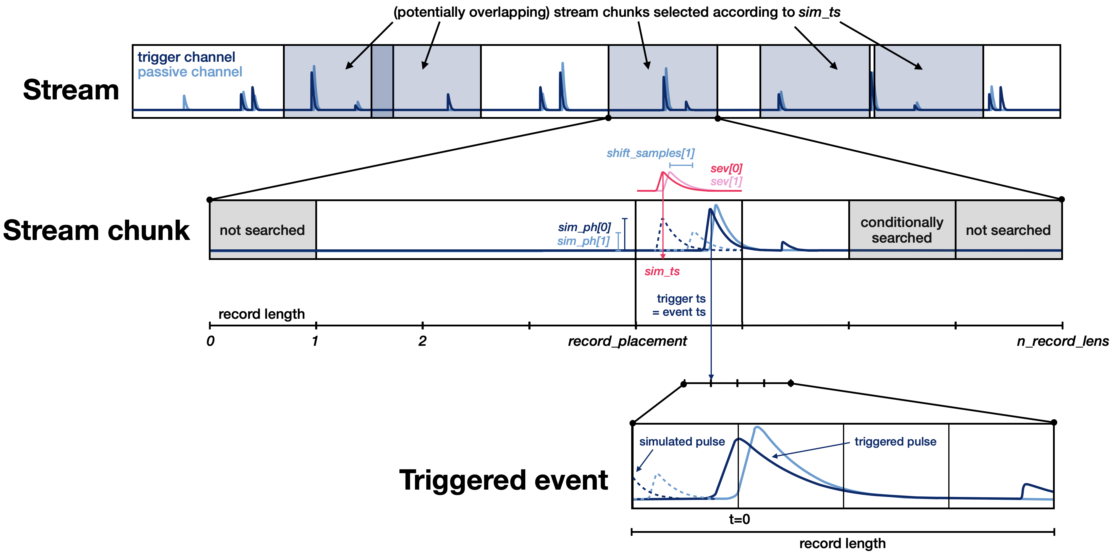
The algorithm described above applies to a single trigger channel. If you trigger multiple, the target index is individually defined for each channel as the maximum of the (non-shifted) SEV of that channel (Note, however, that the simulation timestamp is still defined by the maximum of the (non-shifted) SEV of the first channel). The triggering step is performed for all channels individually. A simulated pulse is considered triggered if either of the channels triggered (i.e. had a trigger within tolerance_samples of the target index). In case more than one channel triggers, the event timestamp is aligned at the maximum of the first channel that triggered (i.e. the first if it triggered, the second if the second triggered but the first one didn’t, etc.).

If testpulse channels are specified, an additional step marks all simulated pulses not triggered if they are within half a record window of a testpulse, regardless of whether they triggered or not. Calibration channel handling for the efficiency calculation is not yet implemented, and can be added in the future if necessary.

Example:

import numpy as np
import scipy as sp

import cait as ai
import cait.versatile as vai

record_length = 2**14
N_sim = 1000

# Set up stream (here just mock, in your case an actual stream)
stream = vai.MockStream(seed=137, rate_Hz=2)

# Set up DataHandler (in your case, you probably have one already)
dh = ai.DataHandler(record_length=record_length, nmbr_channels=2, sample_frequency=stream.sample_frequency)
dh.set_filepath(path_h5="", fname="eff-test", appendix=False)
dh.init_empty()

# You can either use a SEV (array) or fit parameters.
# Here we use fit parameters.
# [t0, An, At, tau_n, tau_in, tau_t]
sev_fitpars = [
    [-2.56, 0.50, 0.50, 3.00, 1.00, 10.00],
    [-2.56, 0.50, 0.50, 0.30, 0.10, 10.00]
]

of = vai.MockData().of[0]

# Random timestamps for simulation (always a good
# idea to sort them so that we don't have to jump
# back and forth in the simulation)
sim_ts = np.sort(
    sp.stats.randint.rvs(
        stream.time[0] + 6*stream.dt_us*record_length,
        stream.time[-1] - 4*stream.dt_us*record_length,
        size=N_sim
    )
)
# Random pulse heights between 0 and 1 (you probably got
# some other range in a real world example)
sim_phs = [
    sp.stats.uniform.rvs(size=N_sim),
    sp.stats.uniform.rvs(size=N_sim),
]
# Random shifts (only for second channel)
shifts = [
    np.zeros(N_sim),
    sp.stats.randint.rvs(-5, 5, size=N_sim)
]

# Run the simulation.
# Note that here, we trigger on Ch0 and Ch1 is read in coincidence.
# Therefore, of must have one channel.
# We still simulate for Ch1, though, meaning that we need sim_phs,
# sev_fitpars, and shift_samples for both Ch0 AND Ch1.
dh.efficiency_sim_trigger_of(
    stream=stream,
    trigger_channels=["Ch0"],
    passive_channels=["Ch1"],
    testpulse_channels=["TP0", "TP1"],
    of=of,
    thresholds=[0.1],
    sim_ts=sim_ts,
    sim_phs=sim_phs,
    #preview=True, # Uncomment to see a preview of the trigger before you run the simulation
    sev_fitpars=sev_fitpars,
    shift_samples=shifts,
)

# Two groups have been created in the DataHandler.
# 'trig-eff-sim' contains trigger information and the
# simulation chunks, 'events-eff-sim' contains the particle
# traces which survived the procedure. Check them out using
dh.content()

# You can look at the stream chunks that were simulated (only contains trigger channels):
vai.Preview(dh.get_event_iterator("trig-eff-sim").with_processing(vai.RemoveBaseline()))

# You can look at the events that survived (contains trigger and passive channels):
vai.Preview(dh.get_event_iterator("events-eff-sim").with_processing(vai.RemoveBaseline()))

# Basic histogram to show what was simulated and what survived.
# You will probably make more sophisticated plots than this.
simulated_phs = dh['trig-eff-sim/simulated_phs', 0]
survived_trigger = dh['trig-eff-sim/flag_survived_trigger']
survived_tp = dh['trig-eff-sim/flag_survived_tp']

vai.Histogram(
    {
        "simulated": simulated_phs,
        "triggered": simulated_phs[survived_trigger],
        "survived tp": simulated_phs[survived_tp*survived_trigger],
    },
    bins=np.linspace(0, 1, 10),
    xlabel="Simulated pulse height (V)"
)

# Have a look at simulated vs. reconstructed pulse heights:
# (Note: reconstructed pulse heights for channels that were not
# triggered are set to -1)
vai.Scatter(
    x=dh["events-eff-sim/simulated_phs", 0],
    y=dh["events-eff-sim/reconstructed_phs", 0],
    xlabel="Simulated pulse heights (V)",
    ylabel="Reconstructed pulse heights (V)",
)

# ... Now you can run additional calculations/cuts on the
# 'events-eff-sim' group and also calculate the cut efficiency.

simulate_pulses(path_sim, size_events=0, size_tp=0, size_noise=0, take_idx=None, ev_ph_intervals=[[0, 1], [0, 1]], ev_discrete_phs=None, name_appendix='', exceptional_sev_naming=None, channels_exceptional_sev=[0], tp_ph_intervals=[[0, 1], [0, 1]], tp_discrete_phs=None, t0_interval=[-20, 20], fake_noise=False, store_of=True, rms_thresholds=[1, 1], lamb=0.01, sample_length=None, assign_labels=[1], start_from_bl_idx=0, saturation=False, reuse_bl=False, pulses_per_bl=1, ps_dev=False, dtype='float32', indiv_tpas=False)

Simulates a data set of pulses by superposing the fitted SEV with fake or real noise.

This method was used to simulate events in “F. Wagner, Machine Learning Methods for the Raw Data Analysis of crypgenic Dark Matter Experiments”, available via https://doi.org/10.34726/hss.2020.77322 (accessed on the 9.7.2021).

Parameters:

• path_sim (string) – The full path where to store the simulated data set.

• size_events (int) – The number of events to simulate; if >0 we need a sev in the hdf5.

• size_tp (int) – The number of testpulses to simulate; if >0 we need a tp-sev in the hdf5.

• size_noise (int) – The number of noise baselines to simulate.

• take_idx (list) – Take only these event indices for the simulation. Overwrites start_from_bl_idx and rms_thresholds.

• ev_ph_intervals (list of NMBR_CHANNELS 2-tuples or lists) – The interval in which the pulse heights are continuously distributed.

• ev_discrete_phs (list of NMBR_CHANNELS lists) – The discrete values, from which the pulse heights are uniformly sampled. If the ph_intervals argument is set, this option will be ignored. This should be one list per channel with have same length. The simulation is done correlated, i.e. the same index from the lists is chosen for all channels. This way e.g. light yields can be simulated.

• name_appendix (string) – A string that is appended to the group name stdevent, which contains the standard event that is used for simulation. This concerns only the simulation of event pulses and has no effect on the test pulses.

• exceptional_sev_naming (string or None) – If set, this is the full group name in the HDF5 set for the sev used for the simulation of events - by setting this, e.g. carrier events can be simulated. Attention! The exceptional standard events are with version 1.0 no longer maintained. Please use the name_appendix argument instead!

• channel_exceptional_sev (list of ints) – The channels for that the exceptional sev is used, e.g. if only for phonon channel, choose [0], if for botch phonon and light, choose [0,1].

• tp_ph_intervals (list of NMBR_CHANNELS 2-tuples or lists) – Analogous to ev_ph_intervals, but for the testpulses.

• tp_discrete_phs (list of NMBR_CHANNELS lists) – Analogous to ev_ph_intervals, but for the testpulses. This should be one list per channel with have same length. The simulation is done correlated, i.e. the same index from the lists is chosen for all channels. This way e.g. light yields can be simulated.

• t0_interval (2-tuple or list) – The interval from which the pulse onset are continuously sampled.

• fake_noise (bool) – If True the noise will be taken not from the measured baselines from the hdf5 set, but simulated.

• store_of (bool) – If True the optimum filter will be saved to the simulated datasets.

• rms_thresholds (list of two floats) – Above which value noise baselines are excluded for the distribution of polynomial coefficients (i.e. a parameter for the fake noise simulation), also a cut parameter for the noise baselines from the h5 set if no fake ones are taken.

• lamb (float) – A parameter for the fake baseline simulation, decrease if calculation time is too long.

• sample_length (float) – The length of one sample in milliseconds (if None, it is calculated from the sample frequency).

• assign_labels (list of ints) – Pre-assign a label to all the simulated events; tp and noise are automatically labeled, the length of the list must match the list channels_exceptional_sev.

• start_from_bl_idx (int) – The index of baselines that is as first taken for simulation.

• saturation (bool) – If true apply the logistics curve to the simulated pulses.

• reuse_bl (bool) – If True the same baselines are used multiple times to have enough of them (use this with care to not have identical copies of events).

• pulses_per_bl (int) – Number of pulses to simulate per one baseline –> gets multiplied to size!!

• ps_dev (bool) – If True the pulse shape parameters are modelled with deviations. Attention! This will always model TUM40-like phonon pulse shapes! The light channel is not affected by this features. Generally, it is not clear how well the deviations model the actual deviations in measured data, so please handle this feature with care.

• dtype (string) – The data format of the simulated raw data events array.

• indiv_tpas (bool) – Write individual TPAs for the all channels. This results in a testpulseamplitude dataset of shape (nmbr_channels, nmbr_testpulses). Otherwise we have (nmbr_testpulses).