Analysis Objects

The classes listed on this page are solutions for reoccurring tasks in an analysis considered more or less ‘standalone’ from the rest of cait. E.g. a standard event (SEV) can exist as an array in isolation (it doesn’t need a cait.DataHandler to be created and it doesn’t have to be saved in one). Likewise, to perform an energy calibration, only arrays of testpulse information are needed (which, of course, can be obtained from a cait.DataHandler). All the classes below have ‘easy-plotting’ built in, i.e. it is very easy to assess the quality of the results, or how the methods work in the first place. Eventually, you will probably save the results into a file or back to a cait.DataHandler, but the point here is that these objects provide you with a playground for trying out things without commitment until you’re happy with the result.

SEV, NPS, NCM, OF, GOF

All these objects are ‘glorified’ numpy-arrays. As such, they can be reshaped, combined to form new arrays, and they carry all typical attributes like .shape, .ndim, …

class cait.versatile.SEV(data: ndarray | IteratorBaseClass = None, dt_us: int = None)[source]

Bases: ArrayWithBenefits

Object representing a Standard Event (SEV). It can either be created by averaging events from an EventIterator, from an np.ndarray or read from a DataHandler or xy-file.

If created from an EventIterator, the (constant) baseline is removed automatically.

Parameters:

data (Union[np.array, Type[IteratorBaseClass]]) – The data to use for the SEV. If None, an empty SEV is created. If np.ndarray (or a list that can be converted to an array), each row in the array is interpreted as a SEV for separate channels. If iterator (possibly from multiple channels) a SEV is calculated by averaging the events returned by the iterator. Defaults to None.
dt_us (int) – The microsecond timebase used in the recording. Only necessary if the input is an array (because it can be automatically inferred if constructed from an EventIterator, a file, or a DataHandler). Defaults to None (i.e. automatic detection if possible).

classmethod from_dh(dh, group: str = 'stdevent', dataset: str = 'event')[source]

Construct SEV from DataHandler.

Parameters:

dh (DataHandler) – The DataHandler instance to read from.
group (str) – The HDF5 group where the SEV is stored.
dataset (str) – The HDF5 dataset where the SEV is stored.

Returns:

Instance of SEV.

Return type:

SEV

classmethod from_file(fname: str, src_dir: str = '')[source]

Construct SEV from xy-file.

Parameters:

fname (str) – Filename to look for (without file-extension)
src_dir (str) – Directory to look in. Defaults to ‘’ which means searching current directory. Optional

Returns:

Instance of SEV.

Return type:

SEV

show(**kwargs)[source]

Plot SEV for all channels. To inspect just one channel, you can index SEV first and call .show on the slice.

Parameters:: kwargs (Any) – Keyword arguments passed on to cait.versatile.Line.

to_dh(dh, group: str = 'stdevent', dataset: str = 'event', **kwargs)[source]

Save SEV to DataHandler.

Parameters:

dh (DataHandler) – The DataHandler instance to write to.
group (str) – The HDF5 group where the SEV should be stored.
dataset (str) – The HDF5 dataset where the SEV should be stored.
kwargs (Any) – Keyword arguments for cait.DataHandler.set().

to_file(fname: str, out_dir: str = '', info_str: str = '')[source]

Write SEV to xy-file.

Parameters:

fname (str) – Filename to use (without file-extension)
out_dir (str) – Directory to write to. Defaults to ‘’ which means writing to current directory. Optional
info_str (str) – An info string to be saved as a description of the SEV in the header of the file. Optional

classmethod unscaled(it: IteratorBaseClass)[source]

Construct SEV from event iterator WITHOUT scaling amplitudes to unity.

Parameters:: it (IteratorBaseClass) – Events from which to construct the SEV.
Returns:: Instance of SEV and relative amplitudes of all channels.
Return type:: Tuple[SEV, np.ndarray]

Example:

import cait.versatile as vai

# Construct mock data to get event iterator
it = vai.MockData().get_event_iterator()

# Get the SEV WITHOUT normalizing (unscaled_sev) and
# the pulse heights (maxima) for all channels.
unscaled_sev, maxima = vai.SEV.unscaled(it)

# With this information, you can construct any desired
# normalization. E.g. the following gives the regular
# SEV, where all channels are normalized to pulse height 1.
regular_sev = unscaled_sev/maxima

# However, if you want to normalize all channels to the first
# channel, e.g., you can do
sev_scaled_to_ch0 = unscaled_sev/maxima[0]

class cait.versatile.NPS(data: ndarray | IteratorBaseClass = None, dt_us: int = None)[source]

Bases: ArrayWithBenefits

Object representing a Noise Power Spectrum (NPS). It can either be created by averaging the Fourier transformed events from an EventIterator, from an np.ndarray or read from a DataHandler or xy-file. If created from an EventIterator, a proper normalisation to physical units (V²/Hz) is performed automatically.

If created from an EventIterator, the (constant) baseline is removed automatically. To improve the quality of the NPS, a window function is often applied to the noise traces before performing the Fourier transform and averaging (see Numerical Recipes by Press, Teukolsky, Vetterling, Flannery chapter 13.4.1). This can only be achieved when we still have the original noise traces, i.e. when we construct the NPS from an iterator. Instead of just a bare iterator it you can pass the iterator it.with_processing([vai.RemoveBaseline(), vai.TukeyWindow()]) to NPS.

Parameters:

data (Union[np.array, Type[IteratorBaseClass]]) – The data to use for the NPS. If None, an empty NPS is created. If np.ndarray, each row in the array is interpreted as an NPS for separate channels. If iterator (possibly from multiple channels) an NPS is calculated by averaging the Fourier transformed events returned by the iterator. Defaults to None.
dt_us (int) – The microsecond timebase used in the recording. Only necessary if the input is an array (because it can be automatically inferred if constructed from an EventIterator, a file, or a DataHandler). Defaults to None (i.e. automatic detection if possible).

classmethod from_dh(dh, group: str = 'noise', dataset: str = 'nps')[source]

Construct NPS from DataHandler.

Parameters:

dh (DataHandler) – The DataHandler instance to read from.
group (str) – The HDF5 group where the NPS is stored.
dataset (str) – The HDF5 dataset where the NPS is stored.

Returns:

Instance of NPS.

Return type:

NPS

classmethod from_file(fname: str, src_dir: str = '')[source]

Construct NPS from xy-file.

Parameters:

fname (str) – Filename to look for (without file-extension)
src_dir (str) – Directory to look in. Defaults to ‘’ which means searching current directory. Optional

Returns:

Instance of NPS.

Return type:

NPS

show(**kwargs)[source]

Plot NPS for all channels. To inspect just one channel, you can index NPS first and call .show on the slice.

Parameters:: kwargs (Any) – Keyword arguments passed on to cait.versatile.Line.

to_dh(dh, group: str = 'noise', dataset: str = 'nps', **kwargs)[source]

Save NPS to DataHandler.

Parameters:

dh (DataHandler) – The DataHandler instance to write to.
group (str) – The HDF5 group where the NPS should be stored.
dataset (str) – The HDF5 dataset where the NPS should be stored.
kwargs (Any) – Keyword arguments for cait.DataHandler.set().

to_file(fname: str, out_dir: str = '', info_str: str = '')[source]

Write NPS to xy-file.

Parameters:

fname (str) – Filename to use (without file-extension)
out_dir (str) – Directory to write to. Defaults to ‘’ which means writing to current directory. Optional
info_str (str) – An info string to be saved as a description of the NPS in the header of the file. Optional

class cait.versatile.NCM(data: ndarray | IteratorBaseClass = None, dt_us: int = None)[source]

Bases: ArrayWithBenefits

Object representing a Noise Covariance Matrix (NCM). The diagonal elements are Noise Power Spectra (NPS) of all channels, while the off-diagonal elements represent the Cross Power Spectra (CPS). The NCM is either constructed from an EventIterator, from an np.ndarray or read from a DataHandler or xy-file. If created from an EventIterator, a proper normalisation to physical units (V²/Hz) is performed automatically.

If created from an EventIterator, the (constant) baseline is removed automatically. To improve the quality of the NCM, a window function is often applied to the noise traces before performing the Fourier transform and averaging (see Numerical Recipes by Press, Teukolsky, Vetterling, Flannery chapter 13.4.1). This can only be achieved when we still have the original noise traces, i.e. when we construct the NCM from an iterator. Instead of just a bare iterator it you can pass the iterator it.with_processing([vai.RemoveBaseline(), vai.TukeyWindow()]) to NCM.

Parameters:

data (Union[np.array, Type[IteratorBaseClass]]) – The data to use for the NCM. If None, an empty NCM is created. If np.ndarray of shape (n_channels, n_channels, n_freq), each diagonal entry (i,i,:) is interpreted as the NPS of channel i, and the off-diagonal elements (i,j,:) correspond to the CPS between channels i and j. If iterator an NCM is calculated by averaging the Fourier transformed events returned by the iterator. Defaults to None.
dt_us (int) – The microsecond timebase used in the recording. Only necessary if the input is an array (because it can be automatically inferred if constructed from an EventIterator, a file, or a DataHandler). Defaults to None (i.e. automatic detection if possible).

classmethod from_dh(dh, group: str = 'noise', dataset: str = 'ncm')[source]

Load NCM from DataHandler.

Parameters:

dh (DataHandler) – The DataHandler instance to read from.
group (str) – The HDF5 group where the NCM is stored.
dataset (str) – The HDF5 dataset where the NCM is stored.

Returns:

Instance of NCM.

Return type:

NCM

classmethod from_file(fname: str, src_dir: str = '')[source]

Load NCM from xy-file.

Parameters:

fname (str) – Filename to look for (without file-extension)
src_dir (str) – Directory to look in. Defaults to ‘’ which means searching current directory. Optional

Returns:

Instance of NCM.

Return type:

NCM

show(**kwargs)[source]

Plot NCM for all channels.

Parameters:: kwargs (Any) – Keyword arguments passed on to cait.versatile.Line.

to_dh(dh, group: str = 'noise', dataset: str = 'ncm', **kwargs)[source]

Save NCM to DataHandler.

Parameters:

dh (DataHandler) – The DataHandler instance to write to.
group (str) – The HDF5 group where the NCM should be stored.
dataset (str) – The HDF5 dataset where the NCM should be stored.
kwargs (Any) – Keyword arguments for cait.DataHandler.set().

to_file(fname: str, out_dir: str = '', info_str: str = '')[source]

Write NCM to xy-file.

Parameters:

fname (str) – Filename to use (without file-extension)
out_dir (str) – Directory to write to. Defaults to ‘’ which means writing to current directory. Optional
info_str (str) – An info string to be saved as a description of the NCM in the header of the file. Optional

class cait.versatile.OF(*args: Any, dt_us: int = None)[source]

Bases: ArrayWithBenefits

Object representing an Optimum Filter (OF). It can either be created from a Standard Event (SEV) and a Noise Power Spectrum (NPS), a SEV and a Noise Covariance Matrix (NCM), from an np.ndarray or read from a DataHandler or xy-file.

Parameters:

args – The data to use for the OF. If None, an empty OF is created. If np.ndarray, each row in the array is interpreted as an OF for separate channels. If instances of SEV and NPS, the OF is calculated from them. If instances of SEV and NCM, the 2d optimum filter (a correlated version of an optimum filter with multiple channels) is calculated. Defaults to None.
dt_us (int) – The microsecond timebase used in the recording. Only necessary if the input is an array (because it can be automatically inferred if constructed from NPS and SEV, a file, or a DataHandler). Defaults to None (i.e. automatic detection if possible).

sev = vai.SEV.from_dh(dh)
nps = vai.NPS.from_dh(dh)
of = vai.OF(sev, nps)

classmethod from_dh(dh, group: str = 'optimumfilter', dataset: str = 'optimumfilter*')[source]

Construct OF from DataHandler.

Parameters:

dh (DataHandler) – The DataHandler instance to read from.
group (str) – The HDF5 group where the OF is stored.
dataset (str) – The HDF5 dataset where the OF is stored. The star * denotes the position of the suffixes ‘_real’ and ‘_imag’.

Returns:

Instance of OF.

Return type:

OF

classmethod from_file(fname: str, src_dir: str = '')[source]

Construct OF from xy-file.

Parameters:

fname (str) – Filename to look for (without file-extension)
out_dir (str) – Directory to look in. Defaults to ‘’ which means searching current directory. Optional

Returns:

Instance of OF.

Return type:

OF

show(**kwargs)[source]

Plot OF for all channels. To inspect just one channel, you can index OF first and call .show on the slice.

Parameters:: kwargs (Any) – Keyword arguments passed on to cait.versatile.Line.

to_dh(dh, group: str = 'optimumfilter', dataset: str = 'optimumfilter*', **kwargs)[source]

Save OF to DataHandler.

Parameters:

dh (DataHandler) – The DataHandler instance to write to.
group (str) – The HDF5 group where the OF should be stored.
dataset (str) – The HDF5 dataset where the OF should be stored. The star * denotes the position of the suffixes ‘_real’ and ‘_imag’.
kwargs (Any) – Keyword arguments for cait.DataHandler.set().

to_file(fname: str, out_dir: str = '', info_str: str = '')[source]

Write OF to xy-file.

Parameters:

fname (str) – Filename to use (without file-extension)
out_dir (str) – Directory to write to. Defaults to ‘’ which means writing to current directory. Optional
info_str (str) – An info string to be saved as a description of the OF in the header of the file. Optional

class cait.versatile.GOF(sev: SEV, nps: NPS, *, basis: str = 'poly', bspec: int | Tuple[List[float], bool] | List[List[float]] = 3, ltc: bool = False, bcc: ndarray = None, window_sev: bool = False, phase: str = '1/4')[source]

Bases: OF

Object representing a generalized optimum filter (see P. Schreiner et al. 2026, to be published).

The generalized filter has to be constructed form a template (SEV) and a noise power spectrum (NPS), as well as a basis which describes the baseline. If you intend to build a traditional optimum filter, use cait.versatile.OF instead.

Note

vai.OF(sev, nps) is equivalent to vai.GOF(sev, nps, basis='poly', bspec=0, phase='argmax').

Warning

If the maximum of your SEV is not aligned at 1/4th of the record window, choosing the correct phase argument (depending on the situation) is important. See below.

Parameters:

sev (SEV) – The template to be used for the filter. Note that only single channel SEVs are supported, i.e. has to be of shape (N,).
nps (NPS) – The noise power spectrum to be used for the filter. Note that only single channel NPSs are supported. Has to have shape (N//2+1,).
basis (str, optional) – The basis for the baseline description to be used. Choose either of poly (polynomial baseline), exp (exponential baseline, plus a constant), or custom (arbitrary basis). The specifics of the corresponding basis are handled by the bspec argument. Defaults to ‘poly’.
bspec (Union[int, Tuple[List[float], bool], List[List[float]]], optional) – Detailed specifications of basis. See table below. Defaults to 3. Together with the default of basis, this corresponds to cubic polynomials.
bcc (np.ndarray, optional) – Basis Coefficient Covariance matrix. If given, the … Has to have shape (K, K), where K is the number of baseline basis vectors. Defaults to None, i.e. implicitly assuming no knowledge about coefficients = infinite variance.
window_sev (bool, optional) – If True, the standard cait.versatile.TukeyWindow is applied to the SEV before filter creation. This might especially be relevant if the SEV does not fully decay inside the record window as it reduces high frequency pollution from the resulting step. Note that applying a window will always increase the minimum possible resolution, but the tradeoff of having less numerical artifacts might be worth it. Defaults to False.
phase (str, optional) – The (complex) phase convention to use in the maximum alignment of the filter. Either of [‘1/4’, ‘argmax’]. See explanation below. Defaults to ‘1/4’.

Baseline model basis functions:

`basis`	`bspec`	Description
‘poly’	0, 1, 2, …	Polynomial degree, e.g. 3 -> cubic baseline.
‘exp’	[tau1, tau2, …]	List of decay constants to consider in the model in seconds.
‘exp_dtau’	[tau1, tau2, …]	Same as ‘exp’ but allows for first order deviations of the time constants from the given values.
‘custom’	[b1, b2, b3, …]	List of arrays which constitute the basis.

Phase argument:

The complex phase (np.exp(-1j*omega*phi), where omega=2*np.pi*np.fft.rfftfreq(sev.shape[-1])) of a filter determines its lag in the time domain. Traditionally, it is chosen such that (in the time domain) the filter output peaks at the maximum position of a pulse. This is achieved with phi=np.argmax(sev).

For finite record windows, the chosen lag acts circularly. You can picture it like moving the SEV in the time domain sample by sample. Samples that fall outside the record window enter again on the other side. For a flat baseline model (which is trivially periodic) and SEVs that decay completely within the record window such shifts usually don’t cause problems. However, if you describe the baseline using non-constant functions (e.g. polynomials) and/or your SEV is non-zero at the end of the record window, this wrap-around is an issue.

There are two cases to consider:

If you just Fourier transform a voltage trace, then multiply it by the filter in frequency domain, then evaluate the result at a fixed sample, the phase is irrelevant as long as the sample where you evaluate it matches the chosen phase. E.g. if you choose phase='argmax' and you evaluate the result at np.argmax(sev), you’re good. Likewise, choosing phase='1/4 and evaluating at sev.shape[-1]//4 is fine.
If you want to slide the filter (like e.g. in cait.versatile.trigger_of() or cait.DataHandler.trigger_of()), the phase has to be zero. Otherwise the wrap-around would spoil the result. For backwards compatibility with traditional OFs (phase aligned with argmax of SEV, usually very close to 1/4th of the record window), those sliding trigger functions automatically account for a phase of 1/4th of the record window! This means that if you intend to use the filter for a sliding trigger, phase='1/4' has to be set when constructing the filter such that it is compensated in the trigger function and the resulting phase is zero again (I agree that this appears cumbersome and confusing, but while implementing this seemed like the best tradeoff between usability, clarity, and backwards compatibility).

Trivially, if np.argmax(sev) == sev.shape[-1]//4, phase arguments ‘1/4’ and ‘argmax’ are equivalent.

`phase`	Use case	Description
‘1/4’	`vai.trigger_of` `dh.trigger_of`	Lag such that it is automatically compensated by sliding trigger functions. Important when triggering with non-constant baselines and SEVs that are non- zero at the end of the window.
‘argmax’	`vai.OptimumFiltering` `dh.apply_of`	Lag such that filter output peaks at SEV maximum. Traditional phase choice. Use for filter output evaluation at fixed sample.

property filter_var: Theoretical variance of the filter’s amplitude estimate.

property filter_var_opt: Theoretical variance of a filter’s amplitude estimate on flat baselines (i.e. if no performance is lost to baseline compensation).

classmethod from_file(fname: str, src_dir: str = '')[source]

Construct GOF from xy-file.

Parameters:

fname (str) – Filename to look for (without file-extension).
out_dir (str, optional) – Directory to look in. Defaults to ‘’ which means searching current directory.

Returns:

Instance of GOF.

Return type:

GOF

to_file(fname: str, out_dir: str = '', info_str: str = '')[source]

Write GOF to xy-file.

Parameters:

fname (str) – Filename to use (without file-extension).
out_dir (str, optional) – Directory to write to. Defaults to ‘’ which means writing to current directory.
info_str (str, optional) – An info string to be saved as a description of the GOF in the header of the file. Defaults to ‘’, i.e. no info string.

Energy Calibration

class cait.versatile.EnergyCalibration(tp_x: ndarray, tp_phs: ndarray, tpas: ndarray, testpulse_response: TestpulseResponse, transfer_function: TransferFunction, max_x_gap: float = inf, param_scale: float = 2.7777777777777777e-10)[source]

Bases: SerializingMixin

Energy calibration for fixed testpulse amplitudes (tpas) and testpulse pulse heights (tp_phs) which vary with an independent variable (tp_x). This independent variable is usually the (microsecond) timestamp of the testpulses but can in principle be any quantity.

NOTICE: The array tp_phs must be cleaned from outliers BEFORE starting the calibration!

Parameters:

tp_x (np.array, shape (N,)) – The independent variable which the testpulse pulse heights tp_phs depend on. Usually the (microsecond) timestamps of the testpulses.
tp_phs (np.array, shape (N,)) – The testpulse pulse heights which vary with tp_x.
tpas (np.array, shape (N,)) – The testpulse amplitudes of each testpulse. This array is used to divide different testpulse amplitudes into separate calibrations.
testpulse_response (TestpulseResponse) – The description for how to fit the set of (tp_x, tp_phs) points (for each TPA individually).
transfer_function (TransferFunction) – The description for how to fit (tpas, tp_phs) values for a fixed x-value.
max_x_gap (float, optional) – If <np.inf, a separate calibration is started if there are gaps in the independent variable tp_x which are larger than this value. Units of max_x_gap are determined by param_scale. Usually, this would be used when tp_x are (microsecond) timestamps and there is no data for > half an hour. In such a case, set max_x_gap=0.5 and param_scale=1e-6/3600. Defaults to np.inf, i.e. this functionality is disabled.
param_scale (float, optional) – Conversion factor between the argument max_x_gap and the units of the input x-values. E.g. If the x-values are given in microseconds, but you want to specify the max_x_gap in hours, you can set param_scale=1e-6/3600. Defaults to 1e-6/3600.

Example:

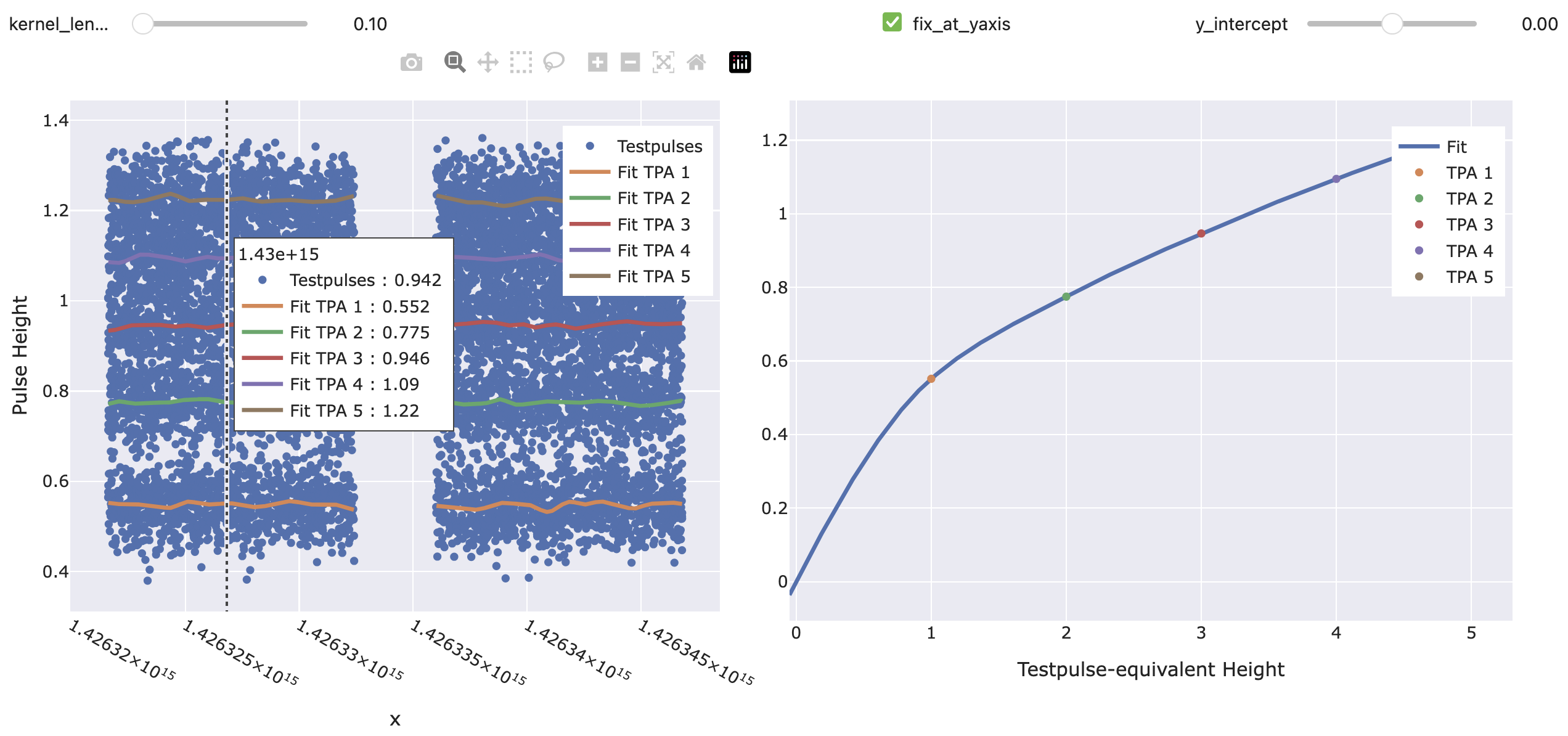
import numpy as np
import scipy as sp
import cait.versatile as vai

# Define a random state (so that this example is reproducible)
rng_seed = 137

# Create mock data. In your analysis, you would of course already
# have timestamps, testpulseamplitudes and testpulse heights.
N = 5000
start_us = 1426321613000000
ts = np.hstack([sp.stats.randint.rvs(low=start_us,
                                    high=start_us+3*1e6*3600,
                                    size=N,
                                    random_state=rng_seed),
                sp.stats.randint.rvs(low=start_us+4*1e6*3600,
                                    high=start_us+7*1e6*3600,
                                    size=N,
                                    random_state=rng_seed)])
tpas = sp.stats.randint.rvs(low=1, high=6, size=2*N, random_state=rng_seed)
tp_phs = sp.stats.norm.rvs(loc=np.sqrt(0.3*tpas), scale=0.05, size=2*N, random_state=rng_seed)

# Create the EnergyCalibration object.
# Choose a testpulse respose object from ['TPRCubicSpline', 'TPRPoly'].
# Choose a transfer function object from ['TFPoly', 'TFPchip'].
# Here, we choose piecewise cubic splines with Gaussian smoothing and
# piecewise cubic Hermite polynomials.
my_ecal = vai.EnergyCalibration(
    tp_x=ts,
    tp_phs=tp_phs,
    tpas=tpas,
    testpulse_response=vai.TPRCubicSpline(kernel_length=0.1),
    transfer_function=vai.TFPchip(),
    max_x_gap=0.5, # start new calibrations for segments which are separated by > 0.5 hours
)

# Open plot that lets you interactively check what your calibration is doing.
# You can change the parameters of the TestpulseResponse and TransferFunction.
# You can click at any time in the left plot to see what the transfer function
# looks like at that time.
my_ecal.preview()

# To convert TPE values to PH values, call the object:
timestamps_of_interest = ts[100:200]
tpes_of_interest = np.linspace(2, 3, len(timestamps_of_interest))
output_phs = my_ecal(timestamps_of_interest, tpes_of_interest)

# To convert PH values to TPE values, call its inverse:
timestamps_of_interest = ts[100:200]
phs_of_interest = output_phs
output_tpes = my_ecal.inverse(timestamps_of_interest, phs_of_interest)

# ... in 'output_tpes' you should have recovered the initial 'tpes_of_interest'.
# Of course, in a real-world scenario, you would only be interested in either
# of the two directions.

__call__(x: ndarray, tpes: ndarray)[source]

Convert testpulse equivalent heights to pulse heights at given x-values (usually timestamps).

Parameters:

x (np.ndarray, shape (N,)) – Independent variable (usually (microsecond) timestamps) for which to evaluate the calibration.
tpes (np.ndarray, shape (N,) or (N, M)) – Testpulse equivalent heights at x-values for which to calculate the pulse height. If 2D, the rows are evaluated at identical x-values.

Returns:

The pulse height for pulses at x with testpulse equivalent heights tpes.

Return type:

np.ndarray, shape (N,) or (N, M)

classmethod from_file(fname: str)[source]

Construct EnergyCalibration from .json-file.

Parameters:: fname (str) – Filename to look for (without file-extension)
Returns:: Instance of EnergyCalibration.
Return type:: EnergyCalibration

get_tp_phs(x: ndarray)[source]

Return the testpulse heights evaluated at x (usually (microsecond) timestamps) for each unique TPA (columns).

Parameters:: x (np.ndarray, shape (N,)) – The independent variable (usually microsecond timestamp) for which to return the testpulse pulse heights.
Returns:: Pulse heights at x for each unique testpulse amplitude (TPA). Invalid values (which fall outside the calibration range) are marked as np.nan. Furthermore, a flag of valid x values is returned.
Return type:: Tuple[np.ndarray, np.ndarray], shape (N, n_unique_tpas) and (N,)

inverse(x: ndarray, phs: ndarray)[source]

Convert pulse heights to testpulse equivalent heights at given x-values (usually timestamps).

Parameters:

x (np.ndarray, shape (N,)) – Independent variable (usually (microsecond) timestamps) for which to evaluate the calibration.
phs (np.ndarray, shape (N,) or (N, M)) – Heights of pulses at x-values for which to calculate the testpulse equivalent height. If 2D, the rows are evaluated at identical times.

Returns:

The testpulse equivalent energies for pulses at x with pulse heights phs.

Return type:

np.ndarray, shape (N,) or (N, M)

plot_testpulse_response(n_fit_grid_points: int = 1000, downsample_factor: int = 1, **viewer_kwargs)[source]

Plot the testpulse response at a given x-value (usually microsecond timestamp).

Parameters:

n_fit_grid_points (int, optional) – Number of points used for plotting the fits. Defaults to 1000.
downsample_factor (int, optional) – Downsample the (tp_x, tp_phs) points by this factor. Defaults to 1, i.e. no downsampling.
viewer_kwargs (Any) – Additional keyword arguments for cait.versatile.plot.viewer.Viewer.

plot_transfer_function(x: float, n_fit_grid_points: int = 1000, **viewer_kwargs)[source]

Plot the testpulse response at a given x-value (usually microsecond timestamp).

Parameters:

x (float) – Number of points used for plotting the fits. Defaults to 1000.
n_fit_grid_points (int, optional) – Number of points used for plotting the fits. Defaults to 1000.
viewer_kwargs (Any) – Additional keyword arguments for cait.versatile.plot.viewer.Viewer.

preview(n_fit_grid_points: int = 1000, downsample_factor: int = 1, **viewer_kwargs)[source]

Plot the testpulse response over time and the transfer function for selected times.

Parameters:

n_fit_grid_points (int, optional) – Number of points used for plotting the fits. Defaults to 1000.
downsample_factor (int, optional) – Downsample the (tp_x, tp_phs) points by this factor. Defaults to 1, i.e. no downsampling.
viewer_kwargs (Any) – Additional keyword arguments for cait.versatile.plot.viewer.Viewer.

to_file(fname: str)[source]

Write EnergyCalibration object to .json-file.

Parameters:: fname (str) – Filename to use (without file-extension)

Testpulse Responses

class cait.versatile.analysisobjects.testpulseresponse.TestpulseResponse(remove_outliers: bool = False, **kwargs)[source]

Bases: SerializingMixin, ABC

Abstract object describing the height of testpulses over x (usually time) for a single testpulse amplitude (TPA).

Parameters:: remove_outliers (bool, optional) – If True, pulse heights that deviate more than 5 sigma from the pulse heights trend will be removed. Note that we always recommend to REMOVE OUTLIERS MANUALLY before even starting the calibration! Defaults to False.

To add a specific model (e.g. piecewise cubic splines or polynomials), the following things need to be implemented:

TestpulseResponse.__init__(): Initialize the object with parameters that it needs (e.g. polynomial order) and call the constructor of the super class with those arguments.
TestpulseResponse.prepare(): Takes a 1-d array of x-values (usually microsecond timestamps) of testpulses of A SINGLE testpulse amplitude and a 1-d array of the corresponding testpulse heights at these x-values (usually timestamps) and performs the fit over x. This method must return the object itself again. Must perform input shape validation, raise a ValueError in case of shape mismatch, and generate a UserWarning if there are outliers in the pulse-heights or less than 10 data points (you can use the function ‘_sanitize_inputs_prepare’ to perform those checks).
TestpulseResponse.__call__(): Takes a 1-d array of x-values (usually microsecond timestamps) and evaluates the polynomial (which was pre-calculated in TestpulseResponse.prepare()). Must perform input shape validation and raise a ValueError in case of shape mismatch (you can use the function ‘_sanitize_inputs_call’ to perform those checks).
If the class attribute _PREVIEW_INPUTS is defined, it will be used for interactively changing the arguments passed to __init__ in the preview methods. See below for how they must be structured. You can only allow a subset of the input arguments to be varied, but all field names in _PREVIEW_INPUTS must be input arguments to __init__.

The usage of this class is demonstrated below for the specific implementation of TPRPoly. See the docstrings of the child classes for more information on the specific behavior.

Example:

import numpy as np
import scipy as sp
import cait.versatile as vai

start_us = 1426321613000000
ts = np.sort(sp.stats.randint.rvs(low=start_us, high=start_us+3*1e6*3600, size=1000))
tp_phs = sp.stats.norm.rvs(loc=1.3, scale=0.05, size=len(ts))

selected_times = np.linspace(start_us, start_us+10000, 100)

# Instantiate the object (this does not yet do any fitting).
tpr = vai.TPRPoly()

# Calculate the fit (this is done only once. Afterwards, the
# object can be used for as many evaluations as you like).
tpr.prepare(ts, tp_phs)

# Get testpulse pulse heights at selected values
tph_at_selected_times = tpr(selected_times)

# Every TestpulseResponse object can be plotted to interactively
# try out different configuration parameters (even before instantiating):
vai.TPRPoly.preview(ts, tp_phs)

abstractmethod __call__(x: ndarray)[source]

Return predicted testpulse heights for given x (usually timestamps).

To use this method, ‘prepare’ has to be called beforehand.

Parameters:: x (np.ndarray, shape (N,)) – Independent variable for where to evaluate the testpulse heights (usually (microsecond) timestamps).
Returns:: Predicted testpulse heights at given x-values.
Return type:: np.ndarray, same shape as x

abstractmethod prepare(x: ndarray, tp_phs: ndarray)[source]

Precalculate the fit over x (usually time) given x-values (usually testpulse timestamps) and testpulse heights.

It is the caller’s responsibility to only pass values corresponding to a single testpulse amplitude (TPA), AND that this data has been cleaned from outliers.

Parameters:

x (np.ndarray, shape (N,)) – Independent variable of testpulses for the calibration (usually (microsecond) timestamps).
tp_phs (np.ndarray, shape (N,)) – Pulse heights of testpulses used for the calibration.

Returns:

This instance.

Return type:

TestpulseResponse

classmethod preview(x: ndarray, tp_phs: ndarray, n_grid_points: int = 1000, **viewer_kwargs)[source]

Plot the testpulses defined by (x, tp_phs) and preview the fit result.

Parameters:

ts (np.ndarray, shape (K,)) – (Microsecond) timestamps of testpulses used for the calibration.
tp_phs (np.ndarray, shape (K,)) – Pulse heights of testpulses used for the calibration.
n_grid_points (int) – Number of points used for plotting the fit.
viewer_kwargs (Any) – Additional keyword arguments for cait.versatile.plot.viewer.Viewer.

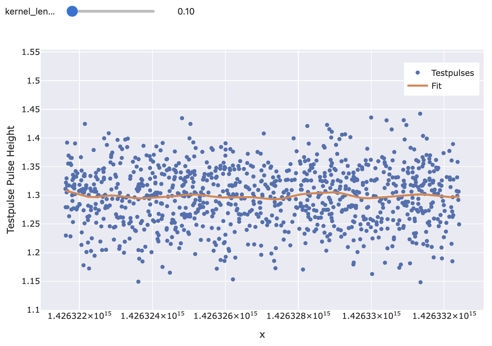
class cait.versatile.TPRCubicSpline(kernel_length: int = 0.5, param_scale: float = 2.7777777777777777e-10, **kwargs)[source]

Bases: TestpulseResponse

Fit testpulse heights with piecewise cubic polynomials. Optionally, Gaussian data smoothing is available before the spline interpolation is performed.

The smoothing can be specified in units different from the x-units using the param_scale argument. I.e. if the x values are microsecond timestamps but you want to specify the smoothing width (kernel length) in terms of hours, you can set param_scale=1e-6/3600 which converts microseconds to hours.

Parameters:

kernel_length (float, optional) – Size of the Gaussian smoothing (1 sigma of the distribution). Units of kernel_length are determined by param_scale. Defaults to 0.5, i.e. with param_scale=1e-6/3600, this corresponds to half an hour.
param_scale (float, optional) – Conversion factor between the argument kernel_length and the units of the input x-values. E.g. If the x-values are given in microseconds, but you want to specify the kernel_length in hours, you can set param_scale=1e-6/3600. Defaults to 1e-6/3600.
kwargs – Additional keyword arguments for see cait.versatile.analysisobjects.testpulseresponse.TestpulseResponse.

This example just demonstrates how the interpolation function looks. For a general description on how to use it, see cait.versatile.analysisobjects.testpulseresponse.TestpulseResponse.

Example:

import numpy as np
import scipy as sp
import cait.versatile as vai

start_us = 1426321613000000
ts = np.sort(sp.stats.randint.rvs(low=start_us, high=start_us+3*1e6*3600, size=1000))
tp_phs = sp.stats.norm.rvs(loc=1.3, scale=0.05, size=len(ts))

vai.TPRCubicSpline.preview(ts, tp_phs)

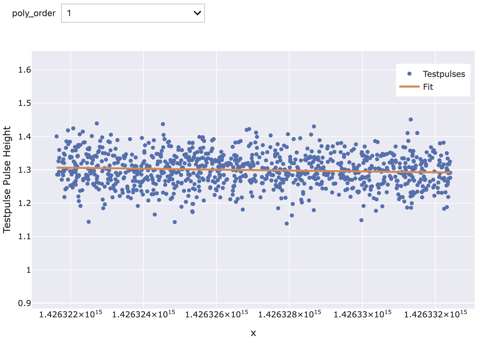
class cait.versatile.TPRPoly(poly_order: int = 1, **kwargs)[source]

Bases: TestpulseResponse

Fit testpulse heights (globally) with a polynomial.

Parameters:

poly_order (Any) – Order of the polynomial. Defaults to 1 (i.e. a linear polynomial).
kwargs – Additional keyword arguments for see cait.versatile.analysisobjects.testpulseresponse.TestpulseResponse.

This example just demonstrates how the interpolation function looks. For a general description on how to use it, see cait.versatile.analysisobjects.testpulseresponse.TestpulseResponse.

Example:

import numpy as np
import scipy as sp
import cait.versatile as vai

start_us = 1426321613000000
ts = np.sort(sp.stats.randint.rvs(low=start_us, high=start_us+3*1e6*3600, size=1000))
tp_phs = sp.stats.norm.rvs(loc=1.3, scale=0.05, size=len(ts))

vai.TPRPoly.preview(ts, tp_phs)

Transfer Functions

class cait.versatile.analysisobjects.transferfunction.TransferFunction(**kwargs)[source]

Bases: SerializingMixin, ABC

Abstract object describing the relation between pulse heights and testpulse equivalent pulse heights. This class is unaware of time, i.e. the interpolation/fit happens in the (TPE, PH)-plane only.

To implement a specific model (e.g. piecewise cubic splines or polynomials), the following things need to be implemented:

TransferFunction.__init__(): Initialize the object with parameters that it needs (e.g. polynomial order) and call the constructor of the super class with those arguments.
TestpulseResponse.__call__(): see its docstring. Must perform input shape validation and raise a ValueError in case of shape mismatch (you can use the function ‘_sanitize_inputs’ to perform those checks).
If the class attribute _PREVIEW_INPUTS is defined, it will be used for interactively changing the arguments passed to __init__ in the preview methods. See below for how they must be structured. You can only allow a subset of the input arguments to be varied, but all field names in _PREVIEW_INPUTS must be input arguments to __init__.

This base class provides a default implementation for TestpulseResponse.inverse(), which calculates the inverse of the fit numerically using the Secant and Bisection Method, given the function TestpulseResponse.__call__(). The class attribute _DEFAULT_ROOT_FIND_ARGS stores the configuration details of this method. If you wish to implement your own inverse (e.g. because there is a more efficient or analytical way to do it) you can override TestpulseResponse.inverse() in the child class. Must perform input shape validation and raise a ValueError in case of shape mismatch (you can use the function ‘_sanitize_inputs’ to perform those checks).

The usage of this class is demonstrated below for the specific implementation of TFPchip. See the docstrings of the child classes for more information on the specific behavior.

Example:

import numpy as np
import scipy as sp
import cait.versatile as vai

tpas = [1.0, 2.5, 4.0, 7.0]
tp_phs_single = [0.8, 1.5, 1.9, 2.3]
tp_phs_multi = [[0.8, 1.3, 1.9, 2.3], [0.7, 1.2, 1.8, 2.4]]
tpes_single = np.linspace(0, 5, 100)
tpes_multi = [np.linspace(0, 5, 100), np.linspace(1, 4, 100)]

tf = vai.TFPchip()

# Evaluate a single calibration (i.e. fit tpas and tp_phs)
# and evaluate this calibration at tpes.
# Shapes: tpas: (n_unique_tpas,)
#         tp_phs: (n_unique_tpas,)
#         tpes: (M,)
#         output: (M,)
ph_values_single = tf(tpas, tp_phs_single, tpes_single)

# Evaluate a multiple calibrations at the same time (i.e. fit
# tpas and rows of tp_phs SEPARATLY, then evaluate each row's
# calibration with each row in tpes).
# Shapes: tpas: (n_unique_tpas,)
#         tp_phs: (N, n_unique_tpas)
#         tpes: (N, M)
#         output: (N, M)
ph_values_multi = tf(tpas, tp_phs_multi, tpes_multi)

# The object also has an inverse method:
# Call tf.inverse() analogously to above to convert from
# pulse height to TPE

# Preview what the transfer function does for different arguments.
tf.preview(tpas, tp_phs_single)

abstractmethod __call__(tpas: ndarray, tp_phs: ndarray, tpes: ndarray)[source]

Calculate pulse height values corresponding to testpulse-equivalent amplitudes tpes, given the testpulse amplitudes tpas and corresponding testpulse pulse heights tp_phs that should be used for the fit.

Parameters:

tpas (np.ndarray, shape (n_unique_tpas,)) – Testpulse amplitudes used for fit. Has to have as many elements as there are unique testpulse amplitudes.
tp_phs (np.ndarray, shape (n_unique_tpas,) or (N, n_unique_tpas)) – Testpulse pulse heights corresponding to tpas. You can pass either as many as there are TPAs or a 2-d array with as many columns as there are TPAs. In the latter case, the fit is performed for each row. See also shape explanation of tp_phs.
tpes (np.ndarray, shape (M,) or (N, M)) – Testpulse-equivalent amplitudes for which to evaluate the calibration. If 2-d, the rows evaluate identical fits.

Returns:

Pulse heights for tpes.

Return type:

np.ndarray, same shape as tpes

inverse(tpas: ndarray, tp_phs: ndarray, phs: ndarray)[source]

Calculate testpulse-equivalent amplitudes corresponding to pulse heights phs, given the testpulse amplitudes tpas and corresponding testpulse pulse heights tp_phs that should be used for the fit.

Parameters:

tpas (np.ndarray, shape (n_unique_tpas,)) – Testpulse amplitudes used for fit. Has to have as many elements as there are unique testpulse amplitudes.
tp_phs (np.ndarray, shape (n_unique_tpas,) or (N, n_unique_tpas)) – Testpulse pulse heights corresponding to tpas. You can pass either as many as there are TPAs or a 2-d array with as many columns as there are TPAs. In the latter case, the fit is performed for each row. See also shape explanation of tp_phs.
phs (np.ndarray, shape (M,) or (N, M)) – Pulse heights for which to evaluate the calibration. If 2-d, the rows evaluate identical fits.

Returns:

Testpulse equivalent amplitudes for phs.

Return type:

np.ndarray, same shape as phs

classmethod preview(tpas: ndarray, tp_phs: ndarray, n_grid_points: int = 100, **viewer_kwargs)[source]

Plot the testpulses defined by (tpas, tp_phs) and preview the fit result.

Parameters:

tpas (np.ndarray, shape (N,)) – Testpulse amplitudes used for the fit.
tp_phs (np.ndarray, shape (N,)) – Pulse heights of testpulses used for the fit.
n_grid_points (int) – Number of points used for plotting the fit.
viewer_kwargs (Any) – Additional keyword arguments for cait.versatile.plot.viewer.Viewer.

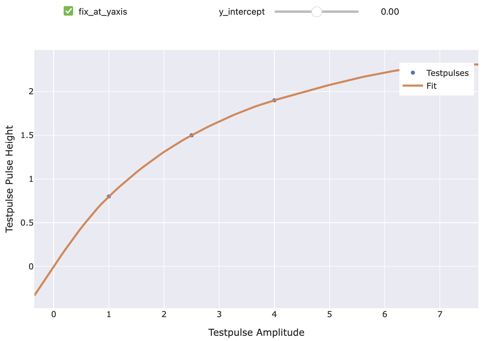
class cait.versatile.TFPchip(fix_at_yaxis: bool = True, y_intercept: float = 0, extrapolate_tangent: bool = True)[source]

Bases: TransferFunction

Transfer function using a Piecewise Cubic Hermite Interpolating Polynomial (monotonic cubic splines).

Parameters:

fix_at_yaxis (bool, optional) – If True, the value when intercepting the y-axis is fixed to the value specified by y_intercept. I.e. when True, the fit considers the additional point (0, y_intercept). Defaults to True.
y_intercept (float, optional) – The y-intercept corresponding to the previous argument. Defaults to 0.
extrapolate_tangent (bool, optional) – If True, values outside the interpolation range (extrapolation) are calculated using the tangent of the polynomial at the last node. This can prevent nonsensical result due to extrapolating cubic polynomials too far. Defaults to True.

This example just demonstrates how the interpolation function looks. For a general description on how to use it, see cait.versatile.analysisobjects.transferfunction.TransferFunction.

Example:

import numpy as np
import scipy as sp
import cait.versatile as vai

tpas = [1.0, 2.5, 4.0, 7.0]
tp_phs = [0.8, 1.5, 1.9, 2.3]

vai.TFPchip().preview(tpas, tp_phs)

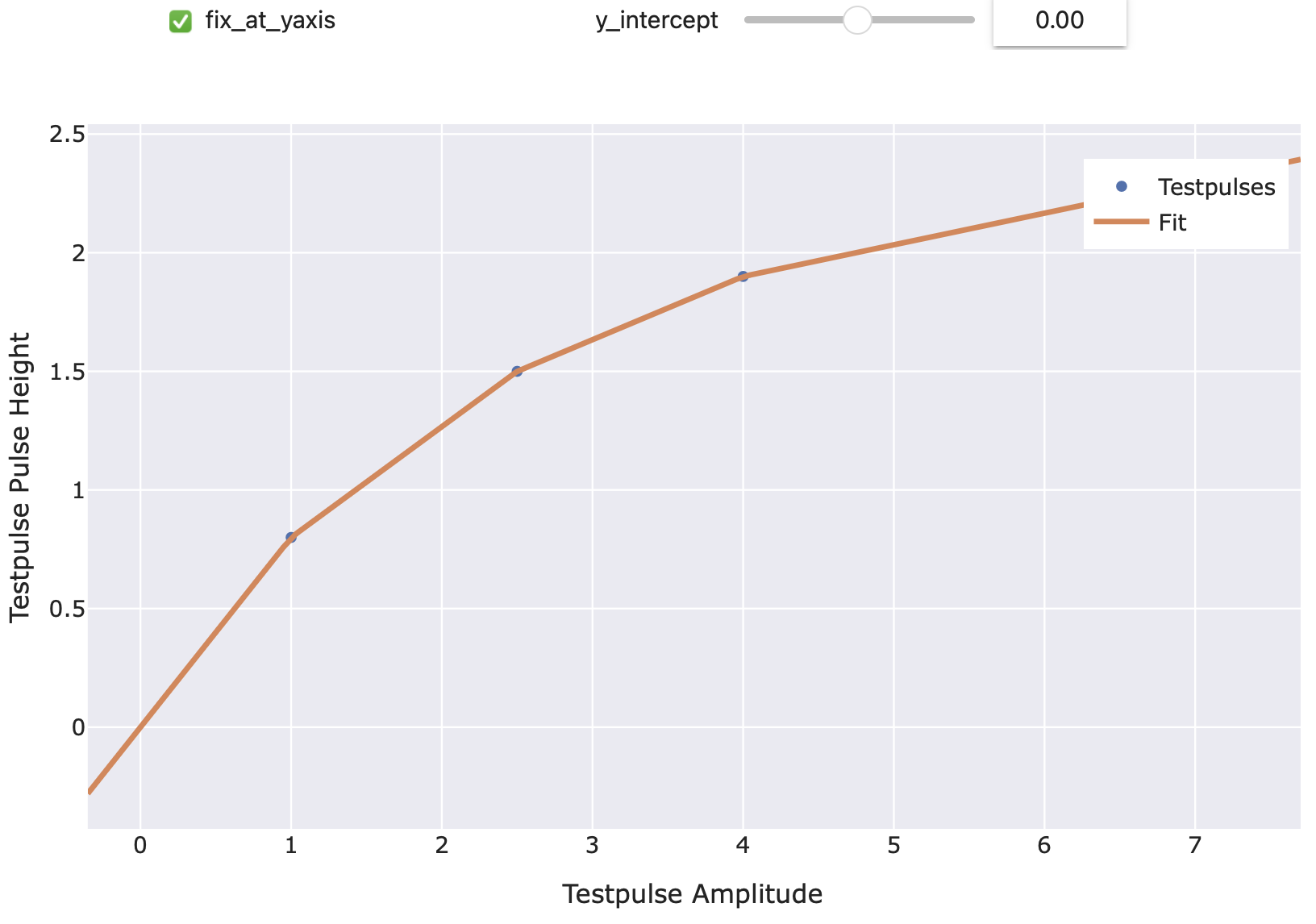
class cait.versatile.TFPlinear(fix_at_yaxis: bool = True, y_intercept: float = 0)[source]

Bases: TransferFunction

Transfer function using a Piecewise linear polynomial.

Parameters:

fix_at_yaxis (bool) – If True, the value when intercepting the y-axis is fixed to the value specified by y_intercept. I.e. when True, the fit considers the additional point (0, y_intercept). Defaults to True.
y_intercept (float) – The y-intercept corresponding to the previous argument. Defaults to 0.

This example just demonstrates how the interpolation function looks. For a general description on how to use it, see cait.versatile.analysisobjects.transferfunction.TransferFunction.

Example:

import numpy as np
import scipy as sp
import cait.versatile as vai

tpas = [1.0, 2.5, 4.0, 7.0]
tp_phs = [0.8, 1.5, 1.9, 2.3]

vai.TFPlinear().preview(tpas, tp_phs)

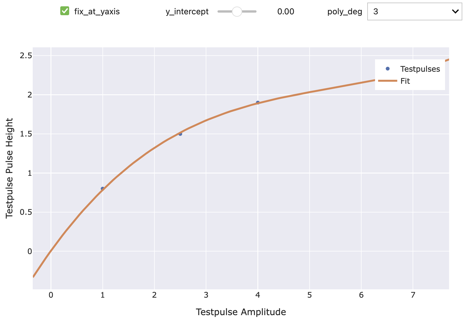
class cait.versatile.TFPoly(poly_deg: int = 3, fix_at_yaxis: bool = True, y_intercept: float = 0)[source]

Bases: TransferFunction

Transfer function using a polynomial.

Parameters:

poly_deg (int) – The degree of the polynomial to use. Defaults to 3.
fix_at_yaxis (bool) – If True, the value when intercepting the y-axis is fixed to the value specified by y_intercept. I.e. when True, the fit considers the point (0, y_intercept) as an additional point. Defaults to True.
y_intercept (float) – The y-intercept corresponding to the previous argument. Defaults to 0.

This example just demonstrates how the interpolation function looks. For a general description on how to use it, see cait.versatile.analysisobjects.transferfunction.TransferFunction.

Example:

import numpy as np
import scipy as sp
import cait.versatile as vai

tpas = [1.0, 2.5, 4.0, 7.0]
tp_phs = [0.8, 1.5, 1.9, 2.3]

vai.TFPoly().preview(tpas, tp_phs)